Data Layers
When the tool opens three dataset layers will display on the map viewer and be listed in the workbench/ navigation pane:
- Place labels
- Coastline/Borders /Roads
- Total Vegetation Cover (the sum of live and dead vegetation and includes trees) as percent cover in the pixel
Turn off any layer by clicking on the white square to the left of the layer title. This will remove the layer from the map view.
Access to data
RaPP Map is a fully open architecture. When you access data through it, you are typically accessing the data directly from the custodian of that data. Data may be updated regularly.
To see the data in more detail, please refer to the Data Catalogue in the RaPP Map itself. Click the Data Catalogue tab and expand the Data Set group names. If you have a dataset you think would suit the RaPP Map then please get in contact with us by emailing geoglam.rapp at csiro.au.
Any information provided by data custodians displayed on the RaPP Map is provided as is and on the understanding that the respective data custodian is not responsible for, nor guarantees the timeliness, accuracy, or completeness of that information. If you intend to rely on any information displayed on the RaPP Map or data.gov.au, then you must apply in writing to the respective data custodian for further authorisation.
You acknowledge that your use of the RaPP Map or data.gov.au means that you have provided your acceptance of these terms and conditions.
Search for data
If you want to search for and add data layers to the RaPP map view you can find available data layers listed in the data catalogue. The data catalogue is separated into Global and National Datasets. Global datasets have an extent across multiple continents, while datasets under the Australia tab may be specific to Australia with an extent equal to or smaller than Australia, for example a single state or territory.
There are three main ways to search the data catalogue:
- Browse the data catalogue – Global and Australia tabs
- Search from the data catalogue tabs search bar
- Search for data from the Search for locations search bar
Browse the data catalogue – Global and Australia tabs
If you want to explore data layers that are available, you can use the Global and Australia tabs.
- Click Explore map data on the Workbench/Navigation pane,
- Select Australia on the top ribbon of the data catalogue window for Australian datasets.
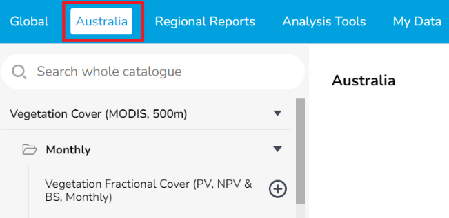
- Data are grouped into themes
- Vegetation cover (MODIS, 500m)
- Vegetation cover – Landat/Sentinel (30/20 meters)
- Land Use / Land Cover
- Landscape attributes
- Boundaries
- Surface water
- Transport
- Expand each theme using the arrow on the right-hand side to see sub-themes and available data layers
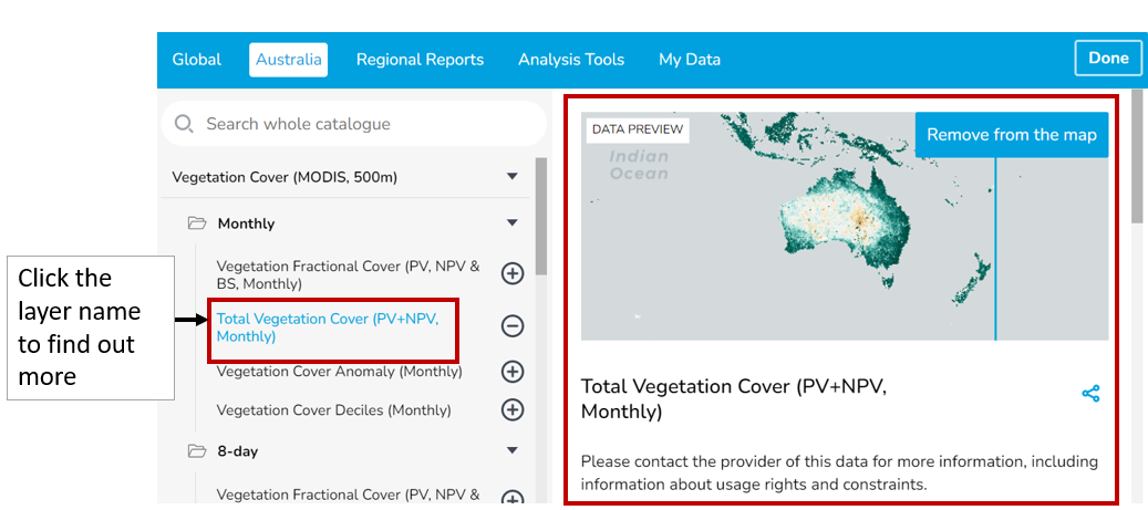
- To learn more about a dataset click the Data layer name. This will display information about the data layer in the right-hand side of the data catalogue window. For data layers open in RaPP map data viewer information about the data layer can also be accessed by clicking About data in the workbench to open the same window.
Search the list from the data catalogue tabs search bar
If you know the name of the data layer you are looking for you can type into the search bar under the Global or Australia tab.
- Open the data catalogue by clicking Explore Map data
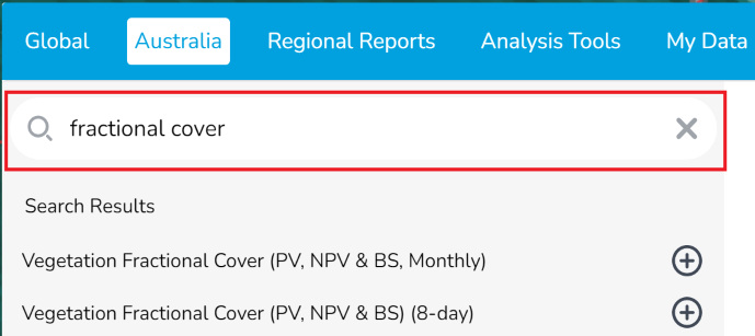
- Type the layer name or keyword into the search bar
- A list of layers matching your search criteria will be returned below the search bar (Figure 21).
- Click layer titles to find out more.
- Click the Plus symbol or add to map to add to the map viewer.
- Click x to clear the search bar.
- Click Done to close the data catalogue window.
Search for data from the Search for locations search bar
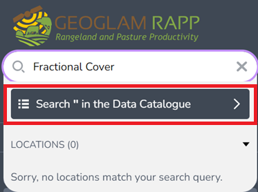
If you know the name of the data layer you are looking for you can also search directly from the Search by locations search bar without opening the data catalogue.
- Type the layer name of keyword into the Search by locations search bar
- Click the black Search “in the Data Catalogue prompt directly below the search bar (Figure 22).
- This will open the data catalogue showing the search returns.
- Click the layer names to find out more. Click + or add to map to display in the map view.
- Click done to close the data catalogue.
Add data and layers
(YouTube video link: 4. Accessing Data Layers - YouTube)
You can add data and layers to RaPP map data viewer from the data catalogue, from your local computer or other web locations (see My data and layers).
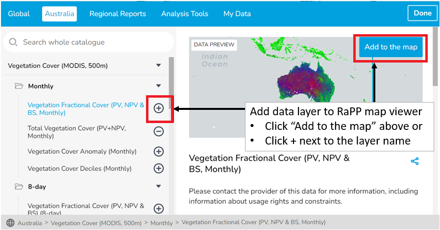
Once you have located a data layer of interest in the data catalogue there are two ways to add the dataset to your RaPP map view (Figure 23):
- Click the Plus symbol next to the data layer name, or
- Click Add to the map in the top right of the dataset metadata You can select the dataset you want from the broad categories from the left side of the window
To add your own data or other public data see My data and layers.
Remove data and layers
There are several ways to remove and hide data layers from the RaPP map view.
-
Removing layers means that they no longer show in the workbench. Layers that have been removed are unavailable for view or analysis. If you wish to use these layers again, they will need to be added again using the same method (section Add data and layers or Data catalogue layers). Removing unused layers is better for analysis.
-
Hidden layers remain in the Workbench but are not shown in the Map view. Hidden layers are simpler to bring back into the Map view. Hiding, re-ordering, or changing layer order are better options for switching between data layer views.
Options to remove data and layers from the RaPP map view
- Remove a single layer using the catalogue
- Remove a single layer using the workbench
- Remove all layers (empty the workbench)
- Return to the default display
Remove a single layer using the catalogue
There are two ways to remove datasets from your RaPP map view using the data catalogue (Figure 24).
- Click the Minus symbol next to the data layer name, or
- Click Remove from the map in the top right of the dataset metadata
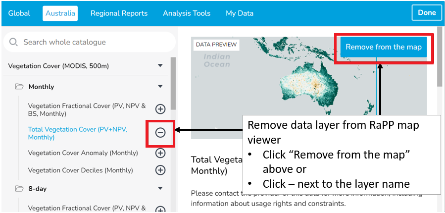
- Click Done to close the Data catalogue window and return to the map view
Remove a single layer using the workbench
To remove a single layer from the workbench
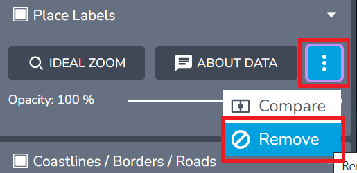
- Locate the layer legend in the workbench legend. If necessary, expand the legend until you can see the three dots icon
- Click the three dots icon
- Click Remove
Remove all layers (empty the workbench)
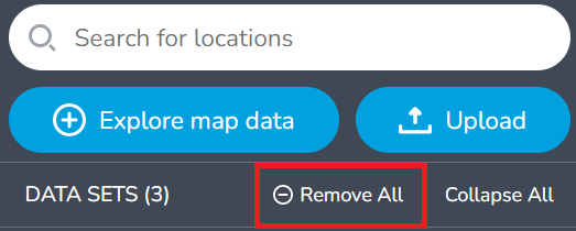
Removing all layers in the workbench area (including the layers loaded by default) will empty the workbench leaving only the basemap. To empty the workbench click Remove All under the blue “Explore map data” and “upload” tools (Figure 26)
Note: All layers will be immediately removed leaving only the basemap. There is no warning or undo for removing all layers. To return to the default view refresh the page or reload GEOGLAM RAPP (geo-rapp.org).
Reordering the layers
To change the order of the layers in the workbench/navigation pane, click a layer and drag it up or down and drop. Reordering the layers is simple and quick way to view what is underneath a particular layer without having to turn it off.
Data with multiple dates
(YouTube video link: 4. Accessing Data Layers - YouTube)
RaPP Map is intended to allow view and analysis of data with multiple different dates. This is also called time series data. For time series data, there are three ways to change the date of the image such as using the time box, the calendar, and the timeline.
Time box arrows
The first time a time series data layer loads it will usually show the latest date in the time box and in the map. The time box can be seen in the workbench when the data legend is expanded (Figure 27).
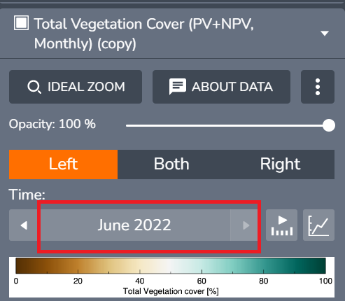
To change the date of data that is displayed in the map view using the time box you can use the time box arrows (Figure 28) or click the time box to select a year and month using the calendar feature (Figure 29 and 30).
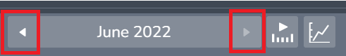
Use the arrows on left and right side of the time box to go to previous and following time periods for this data layer (Figure 28).
Calendar feature
Where there are many time points in the time series data you may wish to choose a non-adjacent time period. For example, for Total vegetation cover (PV+NPV monthly 500m from MODIS) there is data for every month in the record back to 2001). To access other months faster than using the arrows you can click the time box. This will open a dropdown list of years and then a dropdown list of months.
- Click the time box
- Choose a year
- Choose a month
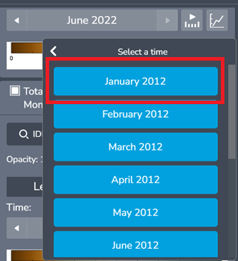
Clicking the time box will open a drop-down list of years, from which then you can select the year you want. For example 2012 (Figure 29). Click anywhere on the line for that year to select it. Note that even though this screen appears to display months within each year you cannot select a month until you progress to the next screen.
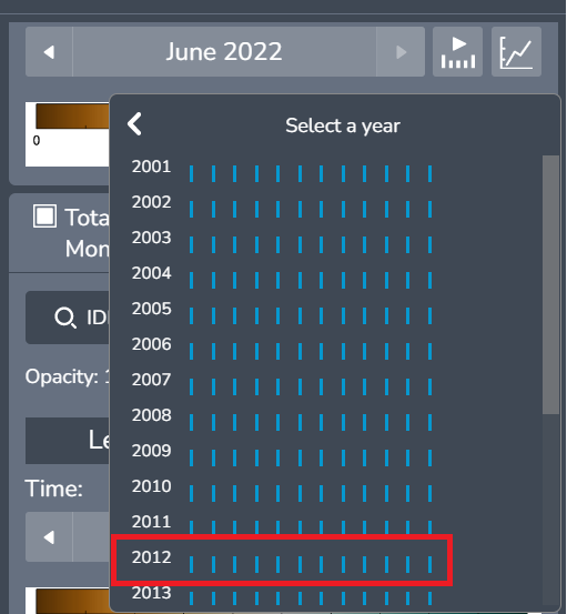
After selecting the year select the month from the new drop down. e.g. “January 2012” (Figure 30). The map display and time box will be updated to this date.
View timeline
(YouTube video link: 3. Workbench - YouTube)
The timeline will add a slider bar to the bottom of the map view. This slider bar can be used to select time periods to display in the map or play a time lapse.
To add the timeline and adjust the date for a time series data layer
- Locate the data layer legend in the Workbench
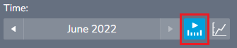
- Click the Use timeline button which has an arrow and 5 bars in it to the right of the date (Figure 31)
- A slider bar appears on the bottom of the map screen.
- Click on the blue balloon (far right of timeline) and slide balloon to the desired date. Once you have selected a new date this will also display in the Time box so you know the date selected

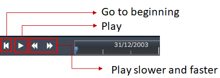
To see the timeseries change from the selected date to present, you can click the play button. The speed of the play can be controlled by the double arrows. Click the pause button to go to the beginning date.
Why is my timeseries change playing very slowly?
This could be because of the high number of loaded layers in the display. Make sure the basemap in 2D mode. Turn off all other unnecessary datasets and run again.
Data catalogue layers
Rapp map comes with a data catalogue containing data layers for view, analysis, reporting and sharing. RaPP map also enables you to add other public data or your own data and layers either from files or web services.
Note that only data catalogue layers will be available to other users if you use the share or story functions (Share, print and Story). Your own layers will not be visible to other users. Your own layers will be removed when refreshing the browser or starting a new session so make sure to download and save any analysis that you have completed before ending your session.
Vegetation cover MODIS 500m
(YouTube video link: 4. Accessing Data Layers - YouTube)
Remotely sensed fractional vegetation cover products separate vegetation into green (photo-synthetic), brown (dry or dead) and bare soil. The RaPP map tool allows you to view fractional cover at different scales from different sensors. Most analysis tools in RaPP map are designed for use with fractional cover products from MODIS at 500m by 500m pixel size. While these pixels are larger than from other sensors the frequency of the product provides tactical information.
- Vegetation Fractional Cover (i.e. shows the green (PV) dead or senescent (NPV) and bare ground fractions)
- Total Vegetation (sum of the green and dead). This layer can be used for time series analysis using points, and polygons (section 5).
- Vegetation cover anomaly (how far the pixel monthly value is away from the mean of the same month from other years)
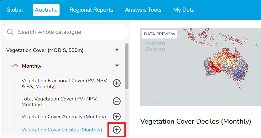
- Vegetation cover deciles (ranking of the pixel monthly value in the record of vegetation cover compared with the same month in other years. Highest (blue) to lowest (red)).
To find these layers in the data catalogue go to:
- Explore map data
- Australia
- Then select the layers under Vegetation Cover (MODIS 500m) by clicking the plus sign on the right-hand side of the layer name
Find persistent low cover areas MODIS 500m
(YouTube video link: 4. Accessing Data Layers - YouTube)
The cover threshold is the amount of Total vegetation cover required to control erosion. The cover threshold indicates whether each pixel is protected from soil erosion.
Different cover thresholds are required to reduce wind or water erosion. Cover thresholds that reduce water erosion (specifically hillslope erosion) vary in different places.
In general, total vegetation cover is recommended to be:
- 50% to control soil loss by wind erosion (Leys 1999)
- 70% or greater to control soil loss by water erosion (Lang 1979). Higher cover thresholds are required on steep slopes (>12%, or 7 degrees), erodible soil types and high rainfall areas.
Cover thresholds apply to a small area or pixel and should not be taken from the average over larger areas or regions.
You can check which part of the country has persistently low ground cover. Go to Explore map data, select Australia and select summaries under the vegetation Cover. Frequency of total vegetation cover data sets are grouped by different percentages (from 30 to 95%) of threshold level of the pixel. For each threshold level, data is grouped in to annual and monthly frequencies.
For example if you want to display the frequency of Total vegetation cover below 50% January
- Click Explore map data, select Australia on the top ribbon of the data catalogue window for Australian datasets.
- Click the drop-down button next to Vegetation Cover (MODIS, 500m) and select summaries.
- Click the drop-down button next to Frequency of Total Veg Cover below 50%
- Click the plus + button next to January – Tot Cov below 50% to load the layer. This shows the frequency of Total vegetation cover equal or lower than 50% in January over the time series.
- Click the legend below the timebox to see the information about the legend in detail.
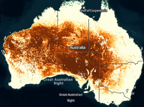
Dark brown colour areas show pixels where Total vegetation cover is more frequently below 50% for the month January over the timeseries.
Vegetation cover deciles
Vegetation cover deciles shows the ranking for the total vegetation cover in each month, in relation to the vegetation cover in that month for all years in the time-series.
-
To add vegetation cover deciles, click the drop-down arrow next to Vegetation Cover (MODIS, 500 m) category to view the available MODIS vegetation cover datasets (For more information see section 6.3.1). Available datasets include
- Monthly: vegetation products derived from imagery collected over the month.
- 8-day: vegetational fractional cover and Total Vegetation cover derived from the 8-day composite imagery
- Summaries: Annual and monthly frequency (in percentage values: 0-100) of Total Vegetation cover lower than various percentages in all months and all years
-
Click the plus + button next to Vegetation Cover Deciles (monthly) to load the layer
-
Now you can see the monthly vegetation decile map on the map viewer display. Select the month and year from the time box, e.g: January 2022.
-
Click the legend below the time box of the layer to see the information about the legend in detail.
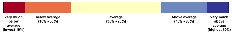
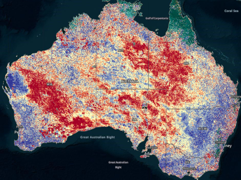
In Figure 37 dark red areas show that in January 2022 these pixels were in the lowest decile of total vegetation cover recorded over the time series for January while dark blue areas are in the highest decile of total vegetation cover recorded over the timeseries for January.
More comprehensive reports of the vegetation cover condition for Natural Resource Management (NRM) Regions and the Local Government Areas (LGAs) can be found in the Regional Reports tab (See Reports for more information).
Contextual layers/Other layers
There are some additional layers in the data catalogue that help understanding the patterns of total vegetation cover.
-
Land use/ land cover
Catchment scale land use and Forest are available. This is a combination of land use data and forest cover data.
-
Landscape Attributes
Landscape Attributes consist layers of physiographic regions, slope and generalised soil order map of Australia.
-
Boundaries
Regions and boundaries are available for Australia. To add a region or boundary file for view or analysis, click Explore map data and select Australia on the top ribbon of the data catalogue window for Australian datasets. Click the drop-down arrow next to Boundaries to view the available boundaries for Australia.
Available boundaries include:
-
Australian Rangelands:
The rangelands are those areas where the rainfall is too low or unreliable and the soils too poor to support regular cropping. They cover about 80% of Australia and include savannas, woodlands, shrublands, grasslands and wetlands. See Australian Collaborative Rangelands Information System (ACRIS) - DCCEEW for more information
-
NRM regions 2017:
NRM Regions is a collective of 54 NRM organisations from all over Australia. See NRM Regions Map – NRM Regions Australia for more information
-
Local Government Areas:
Local Government Areas are an approximation of gazetted local government boundaries as defined by each state and territory. See Local Government Areas | Australian Bureau of Statistics (abs.gov.au) for more information
-
River Regions (Bureau of Meteorology):
Shows National River Basin Boundaries. See Australian Drainage Divisions and River Basin Boundaries: About: Water Information: Bureau of Meteorology (bom.gov.au) for more information.
-
Statistical regions (Australian Bureau of Statistics)
A hierarchy of statistical areas according to ABS Australian Statistical Geography Standard (ASGS). See Australian Statistical Geography Standard (ASGS) Edition 3, July 2021 - June 2026 | Australian Bureau of Statistics (abs.gov.au) for more information.
Unfortunately, you can’t search for individual regions from these boundaries but, once a boundary or region layer is added to and displays on the map you can pan and zoom, and then find out which region a pixel is in by clicking the map and reading the feature information from the pop-up box on the right-hand side of the viewer. You can also navigate to an area of interest using Search for location.
-
Surface Water
Surface water map produced from 25 years of Landsat imagery across Australia is available.
-
Transport
Road layers with national route numbers are available.
I’d love to have a new layer in the data catalogue. Can I suggest?
Absolutely! Just email your suggestion to geoglam.rapp at csiro.au or use the Feedback functionality at the bottom right corner of the map.
My data and layers
(YouTube video link: 5. Understanding Polygons - YouTube)
As well as using the preloaded data layers listed in data catalogue which can be accessed through Explore map data Global and Australia tabs you can upload or add other data to RaPP Map.
You can add your own data from the device you are using with RaPP Map, public web services from other providers, or draw polygons or select points on the RaPP Map viewer.
What can I do with my data and layers uploaded into RaPP map?
- View, pan, zoom
- Show and hide layers
- Change the way uploaded polygons display (style and colour)
- Link CSV files to Australian standard regions and see the data in the map view
- Print map and Print view
- Analysis of time series MODIS fractional cover using your own vector data: points or polygons (see Analysis tools).
What can’t I do with data uploaded into RaPP map?
Data that you upload, polygons you draw, or points you select, will only be available and visible to you during your current session of RaPP map. Uploaded data will not be available or visible once the browser is refreshed, and will not be preserved or made available if you use the following RaPP features:
- Story
- Share
How to upload data
To upload your data into RaPP map you can either:
- Drag and drop the data into the map view, or
- Click Upload from the Workbench.
Follow these steps to upload data from the workbench
- Click Upload or Explore Map data to access the Data catalogue window
- Click My Data
- Find your data. Your data may be local (stored on your device) or web data (available from a URL)
- For local data stored on your device you may prefer to drag and drop. Otherwise click Add Local Data.
- Click Browse to navigate to where your data is stored.
- Select the data you wish to add. Click Open.
- Your data should now be added to RaPP map view, Workspace legend, and details such as the data layer name and extent should show in the data catalogue window.
- Click done on the top right to see your data in the map view.
- For more information about drawing your own polygons see My polygons. For more information about using your polygons for analysis see Analysis tool geometry inputs.
- For web data, click Add Web Data. See Other web services for more information.
- For local data stored on your device you may prefer to drag and drop. Otherwise click Add Local Data.
RaPP map compatible formats for local data include GeoJSON, KML or KMZ, CSV, CZML, GPX, JSON, GeoRSS, glTF, Shapefile (zip) and IFC.
Most of these spatial vector data formats allow you to add points, lines and polygons. There are some differences in functionality. Zipped shapefiles and GeoJSON enable opacity control however KML and KMZ do not.
CSV files
RaPP Map can display two kinds of CSVs/spreadsheets:
- Points
- Data for Australian standard regions.
For more information on special features available with CSV files see the Terria platform user guide https://userguide.terria.io/interactions-functionalities-and-workflows.
Points: To use a CSV spreadsheet to show point locations it will need a point location (latitude and longitude) for each row, expressed as two columns: Lat and Lon. Each row will be displayed as a points or circles at that latitude and longitude.
Data for Australian standard regions: RaPP map allows you to display data on the map for Australian standard regions using a CSV file with rows for each region name. Spreadsheets where each row refers to a region such as a local government area (council), state, postcode, or ABS statistical unit such as an SA2 or CED (Commonwealth Electoral Division) can be displayed on the map. Columns must be named according to the CSV-geo-au standard https://github.com/TerriaJS/nationalmap/wiki/csv-geo-au. Each row will be displayed as a region, highlighting the actual shape of each area.
My polygons
You can use vector polygons or points with analysis tools in RaPP Map. The analysis tools allow you to assess trends over time in Total Vegetation Cover for your area of interest (see Analysis tools).
The analysis on the Total Vegetation Cover Monthly or 8 day data from MODIS. This time series analysis is not available for any other data layers at this stage.
If you have a polygon in a compatible format follow the steps at How to upload data to upload.
If you do not have a polygon but you know the area that you would like to use for analysis there are many ways to create a polygon that you can use in RaPP Map.
Will you need to repeat your analysis, save your polygon, or use elsewhere?
- No – create a point or polygon in RaPP Map see Analysis tool geometry inputs.
- Yes – create and export your polygon using another tool.
RaPP map can accept outputs from most Geographic Information System (GIS) Software such as ArcGIS, QGIS, Google earth etc. If you do not have access to these software you can explore online tools.
This example uses a free online tool that to create a GeoJSON which you can extract for use in other programs such as RaPP. Please note that we do not encourage or endorse the use of this tool over any other tool or suggest that these outputs will meet your needs.
- Go to an online tool for example https://geojson.io/#map=2/20.0/0.0
- Find your area of interest. You can use the search tool in the top right corner to search for a location name. You can click Satellite in the bottom left corner to locate areas using satellite imagery.
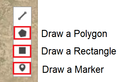
- Click Draw a polygon button
- Click on the corners of the area of interest to see connected lines appearing, click again on the first point to finish creating a polygon. You can also use Draw a rectangular button to “draw a rectangular” polygon and “Draw a marker” button to draw a point
- Once you have created the polygon (or point), click Save on the top ribbon and save as kml or GeoJSON file. (Advantage of GeoJSON file is when it dropped into the Rapp map it will add as a layer with opacity feature where you can set the transparency to see the underneath layer)
- Open Rapp map and add your polygon (See My data and layers).
Edit polygon style
This section explains how to use the style editor to edit the display colour and transparency of polygons imported into RaPP map.
When can I use style editor?
The style editor option should be visible with vector data layers that you have imported into RaPP map (see How to upload data and My polygons). Unfortunately style editor is not available for gridded data or points or polygons drawn directly into RaPP map.
Once you have added your polygon it will be displayed in the map viewer and listed in workbench.
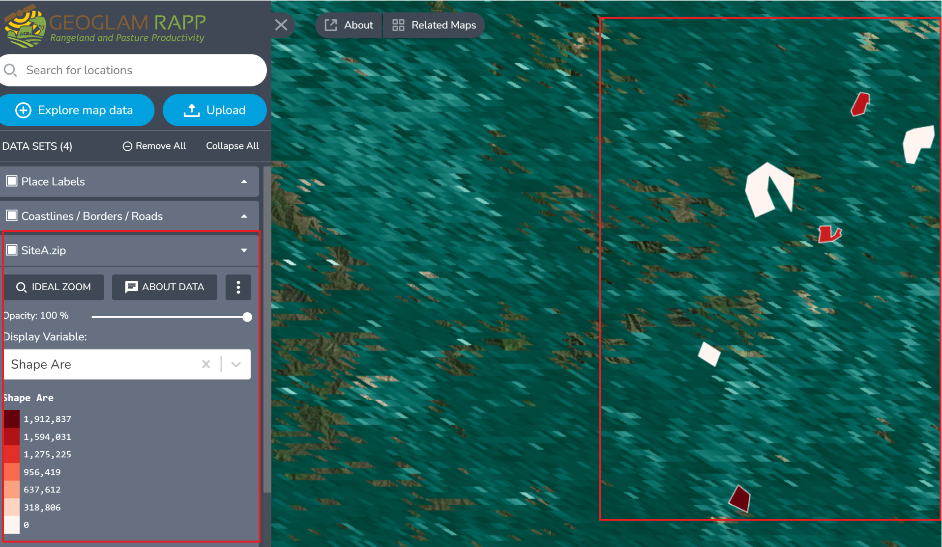
To adjust how your polygon displays you can:
- adjust the slider for opacity
- click the three dots to see Edit style.
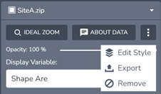
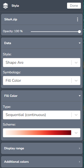
Once you have selected Edit Style, the style editor will open. Using the Style editor dialog box, you can view, create, and modify styles of the polygons.
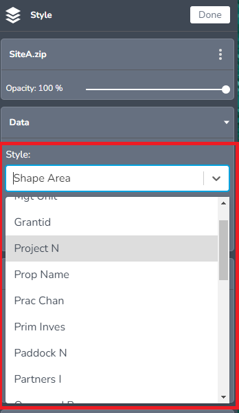
If your polygon data includes distinct categories, such as property name, paddock name, Grant ID etc. you can display those individual categories on the map or you can turn these off to display all in the same way.
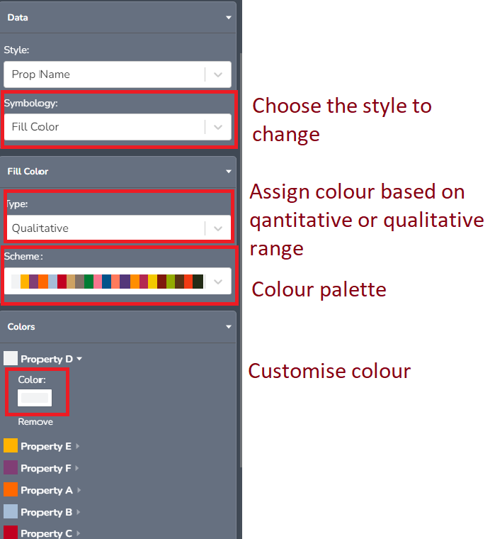
To change the display to relate to a different attribute field:
- Click the small arrow in the text bar below Style and select your category of interest in the style field drop menu.
- Click the Symbology field and choose the polygon style you want to change (eg: Filled colour or outline colour)
- Click the Scheme field and choose a colour palette for the polygons. This will change the color of the polygons on the map viewer to the corresponding category colour.
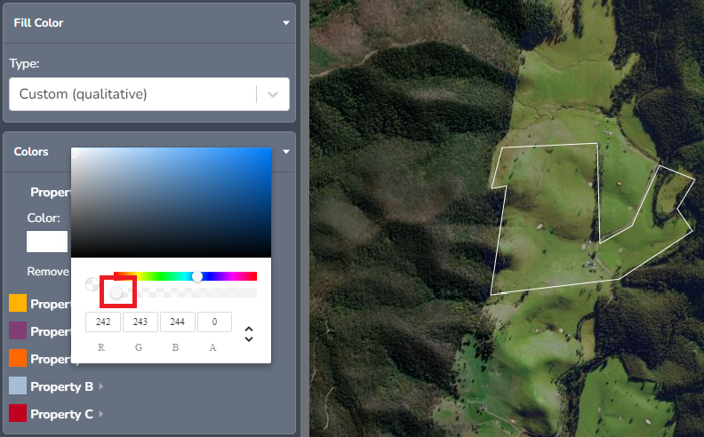
- If you don't find the exact color you want in the array of colors on the Scheme, you can select your preferred colour for each polygon in the colors field. Click the small arrow next to each category (Eg: Property names). Click the colour box. A colour picker window will open. Select the colour you want to choose by one of the below options
- Clicking on the colour scheme Or
- Using the slider box Or
- Typing a colour code into the box.
- Click done at the top right of Style editor to apply your new style.
Note: Unfortunately, you cannot save this style to use in another session. However, you can save and download this view as .png image. See section Print.
You can also use unfilled polygons (only with outline) to view the interior layers. To do this move the slide icon in the transparent slider to the extreme left.
Other web services
You can add any web mapping services from online mapping applications sites.
Web data formats able to be loaded into Rapp map can include Web Map Service (WMS) Server, Web Feature Server (WFS), Esri ArcGIS Server, Esri ArcGIS Map Server, Esri ArcGIS Feature Server,3D Tiles, Open Street Map Server, GeoJSON, KML or KMZ, CSV, Web Map Tile Service (WMTS) Server, Carto, CZML, GPX, GeoRSS, Shapefile (zip), Web Processing Service (WPS) Server, SDMX-JSON, Opendatasoft Portal and Socrata Server.
If the web services layer contains polygon layers (e.g. Boundary layers), they can be used in the analysis. However, raster tiles layers be only used for contextual purposes. They cannot be used for analysis.
For Example, if you want to add Catchment scale land use of Australia 2020 to view the primary land use classes in your target area copy the URL https://www.environment.gov.au/mapping/rest/services/abares/CLUM_50m/MapServer (You can also get this URL from the website https://www.agriculture.gov.au/abares/data/web-mapping-services#web-services-list)
- Click Explore Map data or Upload. Then select My Data tab.
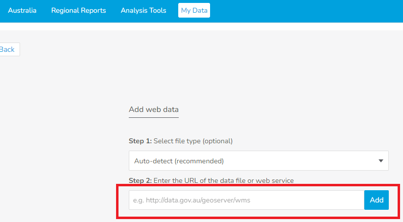
- Click Add Web Data
- Paste the URL you have copied in the Step 2 text box. Click Add.
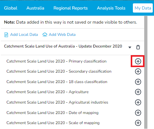
- Click the drop down arrow button next to the data layer name “Catchment Scale Land Use of Australia – Update December 2020” from the left side window. Now you can see the different types of data layers
- Click the plus button next to the data layer “Catchment Scale Land Use 2020 – Primary Classification” to load the data to the Map Viewer. As this is a raster type data layer you can only use this for contextual purposes.