Chapter 5
	Dynamic Water Balance Modelling
	Sections 5.1 and 5.2 (5.2.1 to 5.2.3)

Topog_Dynamic is a fully transient water balance model. As with the steady-state module Topog_Simul, this transient module operates on the same element network generated by Topog_Element.

Topog_Dynamic can be run either as a daily timestep 'yield' model or as a sub-daily timestep 'stormflow' model. In the 'yield' mode solute transport and vegetation growth can also be accounted for. In the 'stormflow' mode kinematic wave overland flow and sediment transport can be simulated. Evapotranspiration is not calculated when the model is run in 'stormflow' mode.

Processes simulated by Topog_Dynamic (not necessarily all at once) include:

• interception of rainfall by plants and evaporation of water from the canopy (up to 2 plant layers) and bare soil surfaces.

• infiltration and vertical redistribution of soil water.

• the dynamics of perched water tables and the lateral movement of soil water in the saturated zone.

• transpiration and soil water uptake by plants (up to 2 plant layers).

• plant growth, comprising carbon allocation to roots, leaves and stems of plants (up to 2 plant layers).

• recharge to and discharge from a groundwater store.

• salt transport in the soil.

• overland flow height, velocity and flux.

• sediment detachment, transport and deposition.

Computations in Topog_Dynamic are performed in:

• a soil water module
• an evapotranspiration module
• a plant growth module
• a solute transport module
• an overland flow module
• a sediment transport module

Brief descriptions of each of these modules are given below.

5.2.1 The soil water module

The soil water module accounts for infiltration and vertical percolation of water through the unsaturated zone, and lateral movement of water in the saturated zone. Topog_Dynamic supports three different soil water accounting schemes, these being :

• Newton-Raphson scheme (NR) (an implicit solution of the Richards equation)

• Runge-Kutta scheme (RK) (an explicit solution of the Richards equation)

• the Simplified Bucket Model scheme (SBM)

All three schemes can be used in the 'yield' and 'stormflow' modes, though solute transport is only linked to the NR scheme and sediment transport is only linked to the SBM scheme.

The NR and RK schemes allow for soil layering, whereas the SBM scheme assumes a single layer of soil where the hydraulic conductivity decays exponentially with depth. In the NR scheme, soil moisture is computed at a stacked series of 'nodes'; in the RK scheme, computations are made for a stacked series of 'compartments'. When a water table develops at any node (using the NR scheme) or in any compartment (using the RK scheme), water is routed downslope through the Topog flow net using Darcy's law (i.e. at a rate based on the local soil Ks value and the slope of the saturated water surface, assumed to be the same as the topographic gradient).

As in Ross (1990), the NR scheme adopts the 'Kirchoff transform' to reduce the spatial and temporal nonlinearity of the suction (y), and uses the 'mixed' form of the Richard's equation, as it has much better mass conservation in numerical form than the pure potential form. The adopted form of the Richards equation is:

dq dt = d dz [ K - dU dz ]

5.1

where

q = soil moisture content (a function of z and t)
t = time
z = depth from the surface
K = soil hydraulic conductivity, and
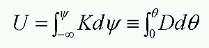
U = the Kirchoff transform variable, calculated as:

5.2

where:

y = the soil water pressure potential, and this also defines D the diffusivity.

Allowance has been made for up to 8 different layers to be ascribed to any soil profile, and the organisation of layers is permitted to vary between adjacent catchment elements. It is assumed that that soils are isotropic and that no hysteresis occurs.

The SBM scheme is based on the TOPMODEL concept (Beven and Kirkby, 1979). A basic assumption of this scheme is that soil hydraulic conductivity (Ks) declines exponentially with depth, according to:

Ks = K0 exp(f/z)

5.3

where:

K₀ = the saturated hydraulic conductivity at the surface
z = the depth into the soil
f = -mDq

and where:
m = a constant which controls the hydrograph recession shape
Dq = the volumetric soil moisture deficit below saturation

Using the SBM scheme, subsurface lateral flow (q_l) out of any catchment element i runs downslope between flow trajectories according to:

ql = Ki tan(b) exp (Si/m)

5.4

assuming:

b = the element slope angle
m > 0
K_i = the soil hydraulic conductivity (K_s) of the element, assuming the element soil moisture storage deficit (S_i) to be zero.

The exponential term in Eq 4 is bounded by @ 0 <= exp(S_i/m) <= 1. Hence when m=0, equation 5.4 is changed to:

ql = Ki tan(b) saturated storage/actual storage

5.5

to ensure no lateral subsurface flow occurs when the element is dry.

The soil moisture dynamics module also includes a simple macropore flow algorithm. Each element is ascribed :

a macropore volume (M_d)
a macropore depth (M_z)
a macropore saturated hydraulic conductivity (M_ks)

The macropore is permitted to fill only when infiltration excess occurs, ie. the rainfall intensity exceeds the infiltration capacity of the soil, or the soil profile is saturated. At the end of each timestep, lateral flow is allowed to occur via macropores at a rate governed by the topographic slope and M_ks. Flow is permitted between the macropore and the matrix at a rate governed by the instantaneous hydraulic conductivity of the soil matrix (m_k). See the notes on Topog_Soil for more information on the macropore flow option.

5.2.2 Solute transport

The soil column conservative solute transport is described by the convection-diffusion equation in 1-dimension :

d(qc) dt = d dz { q Dzz dc dz } - d(qwc) dz

5.6

where:

c = the solute concentration
D_zz = vertical component of the hydrodynamic dispersion tensor
q_w = the vertical water flux

This can be rewritten as:

d(qc) dt = dqs dz

5.7

where now the solute flux, q_s, is :

qs = q Dzz dc dz - qwc

5.8

5.2.3 The evapotranspiration module

Transpiration from the overstorey and understorey vegetation, and evaporation from the soil/litter layer is predicted for each catchment element at each timestep when the model is run in 'yield' mode. For each of these layers, the surface radiation balance consists of four components:

• incoming short-wave radiation (the driving variable)
• reflected short-wave radiation from the surface
• incoming long-wave radiation from the atmosphere
• emitted long-wave radiation from the surface

Short-wave downward radiation on a horizontal surface is modified across the catchment according to the slope and aspect of each computational element (Klein, 1977). This is accomplished by supplying the model with a radiation coefficients table, generated with the programme Topog_Rcoeff.

From both canopies the Penman-Monteith equation is used to compute transpiration:

lE = s Rn + r Cp Da/ra (s + g( 1 + rs/ra))

5.9

where:

s = the slope of the saturation vapour pressure-temperature curve
R_n = net radiation
r = the air density
C_p = the specific heat of air
D_a = the vapour pressure deficit (VPD) of the air above the canopy
g = the psychometric constant
r_a = the aerodynamic resistance, and
r_s = the canopy (surface) resistance

The transpiration model can use two different representations of canopy conductance, g_c, determined for each canopy layer:

1. A maximum canopy conductance is specified for each vegetation layer and this value is scaled down linearly according to the vapour pressure deficit (Running and Coghlan, 1990)

   gc = gmax Y* (1-Dvpd Dc)

   5.10

   where:

   g_max = the maximum canopy conductance
   y^* = -y_mean/y_lwmax is a normalised moisture stress index
   y_mean = the mean soil moisture potential within the soil column
   y_lwmax = the maximum (most negative) leaf water potential of the canopy
   D_vpd = the slope of the g_c response to vapour pressure deficit
   D_c = the vapour pressure deficit in the canopy air
   

2. The canopy conductance is proportional to the carbon assimilation rate, and modified by the surrounding air vapour pressure deficit, following Ball et al. (1987) as modified by Leuning (1993):

   gc = g0 + g1 A / [ ( Cs - G ) (1 + Dc Dco ) ].

   5.11

   where:

   g₀ = the minimum canopy conductance
   g₁ = the slope of the conductance dependence on VPD
   A = the carbon assimilation rate discussed in the growth module section
   C_s = the atmospheric CO₂ concentration
   G = the CO₂ compensation point
   D_co = an empirical coefficient
   

3. The canopy conductance is proportional to assimilation rate and is moderated by transpiration rate, as discussed by Monteith (1995) and implemented by Slavich et al (in prep).

   gc = 1.6 [ (1+1/W) Amax XW XE (1 - e-k LAI) ] (Cs - G) Dl

   5.12

   where:

   W =	the ratio of the maximum liquid phase mesophyll conductance to the maximum gas phase stomatal conductance (0.2 for C3 plants and 0.8 for C4)

   
   A_max = the maximum carbon assimilation rate
   

   X_W, X_E are normalised stress indices for water availability and leaf transpiration rate (discussed below)
   

   k = the light extinction coefficient of the canopy
   LAI = the leaf area index of the canopy, and
   D_l = the day length in seconds
   

   The factor 1.6 is the ratio of the diffusion rates of CO₂ and water vapour.

The vapour pressure deficit at each canopy (D_c) and at the soil surface is calculated using the omega decoupling coefficient (W_c) proposed by Jarvis and McNaughton (1986).

Dc=Wc Deq+(1-Wc)Da

5.13

where:

D_eq = the equilibrium VPD given by:

Deq= g e Rn Cp gc (e+1)

5.14

and: e = s/g

Soil evaporation is calculated using the Penman-Monteith equation with the surface resistance set to zero if the soil surface is not air-dry, or determined by the method of Choudhury and Monteith (1988) when in second phase drying:

rs = t l h Dm

5.15

where:

h = the porosity of the soil
D_m = the molecular diffusion coefficient for water vapour
t = a tortuosity factor and l is the depth of the air-dry soil layer