
|
|
|
Chapter 4 |
|
Steady State Water Balance Modelling |
|
Sections 4.1 to 4.3 |
4.1 |
Background |
Topog_Simul performs a suite of steady-state hydrologic simulations.
To run Topog_Simul, type: $ _simuland supply the basename of your catchment when prompted. The program first reads in the catchment dimensions (.sys) file, then the terrain attributes (.atr) and element connection (.cct) files. The user then has the choice of eight different steady-state simulation options. These are listed in the Topog_Simul menu as shown below:
These eight options can be classified into two broad classes. The steady-state drainage index and the radiation weighted drainage index (options 1 and 2) can be classified as soil wetness indices. The uniform and variable excess stream power options, the shear stress options and the erosion hazard options (options 3 to 8) can be classified as erosion hazard indices.
Results from each of these simulations are written to files with specific extensions. Because they contain spatial data every output file has both a basename and a qualifier. The extensions are listed in Table 4.1 below. Also summarised in this table are the abbreviations used for each option and the computational units used.
Table 4.1 List of abbreviations and units used for the various attributes computed using Topog_Simul. Also shown are the filename extensions used for results files. [ ] denotes the unit is dimensionless.
Simulation option Symbol Unit Extension Steady-state drainage index W [ ] .ssd Radiation-weighted drainage index Wr [ ] .rwd Uniform excess stream power Pu W/m2 .usp Variable excess stream power Pv W/m2 .vsp Erosion hazard index H W/m2 .ehi Saturation Flow shear stress tb dynes/cm2 .sss Hortonian shear stress tb dynes/cm2 .hss Landslide hazard index qcr mm/day .lhi
4.2 |
The steady-state drainage index |
The drainage capacity of any point in the landscape is affected by its slope, the size of its source area, its evaporation rate (primarily a function of slope and aspect) and its soil transmissivity. The drainage index is a measure of each element's ability to drain a prescribed net lateral drainage flux (q), taking into account the factors mentioned above. The quantity q is defined as the residual of rainfall (R) once evaporation (E) and deep vertical drainage (D) are subtracted (i.e.: q = R-E-D). Conceptually, q can be thought of as the catchment baseflow; the water balance component which moves slowly downslope through the soil.The drainage index (W) for each element ((x,y)) is calculated by Topog_Simul in the following way:
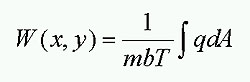
4.1 where
m = slope (m/m)
b = length of contour at base of element (m)
T = local transmissivity (m2/d)
A = element area (m2)
q = net subsurface drainage flux (m/d). In computing this quantity across the catchment, spatially variable values of T and q can be used. The resulting W index is dimensionless; a value of one or more represents soil saturation. To perform this simulation, select option 1 from the main menu:
As part of the operation of Topog_Simul, a summary table of simulation results is produced. The table uses default classes.
Topog_Simul asks for information on soil transmissivity. If variable T values are to be used, then you must supply the name of a file containing a T value for each element in the network (in this case we have a file called yahoo.tvals). This type of file is created using Topog_Overlay. If you are assuming a uniform T value for the whole catchment, enter a < Return > and the program will prompt you for that single value. Most T values lie in the range of 0.01 to 10 m2/d.
Enter filename of transmissivity (< CR >=NONE) : yahoo.tvals
Simul: Reading file "yahoo.tvals" ....
After the soils information is read in you are asked to enter the q value (referred to here as baseflow). You have the option to distribute variable q values over the catchment; this could be done to reflect the effect of different vegetation. If you do not have variable data, press < Return > you will then be required to supply a single q value for the whole catchment. In the example below we will use a value of 0.1 mm/d for the entire catchment. Most catchment baseflows would lie in the region of 0 to 10 mm/d.
Enter filename of subsurface drainage flux (< CR >=NONE) :_
Enter uniform subsurface drainage flux (mm/day): .1
Next you are given the option to impose the effect of line sources or line sinks in the element network.
Filename of line sources ( =NONE) : _ With the sources/sinks option you can specify a line along any segment of contour in the element network from which water is either pumped out or trapped. Several sources and sinks can be specified across the landscape. To use this option a line sources/sinks file must be supplied containing information on line source/sink location(s). The conventional (though not mandatory) extension for such a file is .lines. The .lines file is a free format file which (for each line source/sink) specifies:
contour number on which the line source/sink resides
start element number finish element number
source output quantity (m3/day) -OR- sink efficiency fraction (-1 to 0)This pattern may be continued for as many line sources or line sinks as required. No blank lines are permitted in this file. If the contour number is out of range, the next two lines are ignored. If the first element number is less than 1, it is set to 1. If the last element number is greater than the number of elements on this contour, it is set to the maximum. So if you wanted to specify the whole contour as a line source or sink you would use 1 and 9999 as the first and last element numbers. If the last element number is less than first element number, then they are swapped. A sink efficiency value of -1 will trap all flow from upslope, a value of -0.5 will trap 50% of that flow. Both source and sink terms are distributed equally along the length of contour specified by the user. If you do not want to utilise this option, simply press < Return >.
The user is then given the option to alter the direction of flow across the element network.
Enter redistribution filename ( = NONE): With the redistribution option you can modify the flow connectivity to account for banks, roadways, drains and preferred flowpaths. The redirection file is created using the utility program Topog_Redflow.
At this stage, Topog_Simul computes the steady-state drainage index for each catchment element and outputs results in the following format:
Baseflow recorded =            0.0071 mm/d
Bankflow recorded =            0.0000 mm/d
Stream q recorded =            0.0929 mm/d
Drain q recorded  =            0.0000 mm/d
  5.82 seconds elapsed

Resulting classes as % catchment area
	   RANGE               %
    Less than  0.1250E+00    20.71
 0.1250E+00 -  0.2500E+00    18.13
 0.2500E+00 -  0.5000E+00    18.61
 0.5000E+00 -  0.1000E+01    15.47
 0.1000E+01 -  0.2000E+01     9.97
 0.2000E+01 -  0.4000E+01     7.09
 0.4000E+01 -  0.8000E+01     2.55
 0.8000E+01 or more           7.48

Save these results ? (Y/N)         [N] : y

Writing result file "yahoo_a.ssd" ....
For this simulation, over 27% of the catchment area was calculated to be saturated (i.e.: over 27% of the catchment area had W > 1). When the computation is complete, you have the option to write the results to a file or discard them.
Save these results ? (Y/N) [N] : y In this case, simulation results are written automatically to a file called yahoo_a.ssd. If there was already a file with this name in the operative directory, Topog_Simul would have detected this and changed the qualifier to the next letter in the alphabet (i.e.: to yahoo_b.ssd). All of the input particulars and the table summary shown above are written to the top of the .ssd file as a header. If line sources or line sinks were used then a .lns file is also written (using the same qualifier). This is a flat format file which is used to display the position of the line sources and line sinks used. After all of the files are written to disk, you have the option to run another simulation or quit from Topog_Simul.
Run another simulation? (Y/N) [N] : y
4.3 |
The radiation-weighted drainage index |
The radiation-weighted drainage index (Wr) is a variant of the normal drainage index described in the previous section. In the last simulation, evaporation rate (E) was assumed to be uniform across the catchment. However, Topog can automatically calculate the potential solar radiation for each element for any time of the year, giving us the capability to distribute evaporation variably across the catchment. The index assumes that evaporation is a function of the amount of radiation and the cube-root of soil moisture (i.e.: W is used as a surrogate for soil moisture). A cube-root function is used because a linear weighting fails to recognise that efficiency is high until soil moisture is quite low.The simulation is performed in the same manner as the normal drainage index, except the user is prompted for three additional inputs, these being the EFT parameter, EFS parameter and solar declination. The EFT term represents the efficiency of transpiration on a given element (where the radiation varies according to the aspect and slope of the element). It is used to scale down potential solar radiation because much of this energy is attenuated by clouds and dust in the atmosphere, and even with clear sky, only a fraction of solar radiation is converted into net radiant energy. The EFT term is difficult to properly quantify (particularly in a steady-state sense), but it is recommended that you adopt the default setting, which is 0.25. The EFS term is similar, but is the fraction applied to a shaded horizontal surface. This is also dificult to quantity, but we recommend that you use the default setting of 0.02.
The Wr index is calculated as in equation (4.1), except that a transpiration-modulated drainage flux (qe(x,y)) is calculated. Thus:
qe(x,y) = R - [( a rs (x,y)
2.2248+ b rh
2.2248) *W1/3 ] - D 4.2 where a is the EFT term used to scale the total solar radiation for each element (rs(x,y)) and b is the EFS term used to scale the total solar radiation on a horizontal surface (rh) in a shaded state. The value of 2.2248 is a conversion factor to change radiation units (MJ/m2/day) to equivalent transpiration units (mm/d). As defined earlier, R is the net rainfall (mm) and D is deep drainage (mm).
Equation (4.2) shows that qe(x,y) depends on W, which is in turn dependant on the area integral of q. Hence, W is calculated by iteration until stable values of Wr and qe are obtained.
As in the normal steady-state drainage index simulation, polygonal overlays of T, R, and a can be used, and lines sources, sinks, and redirection flow can be imposed. Results of a radiation-weighted drainage index computation are written to a .rwd file. This file also contains a header listing all of the input parameters and files used.
| Take me out of frames | Chapter 4 continued....... |