 |
Chapter 3 ....continued
|
|
Chapter 3 ....continued
|
3.6 |
Building the .hpt, .sad, .stl and .vrt files automatically |
The .hpt, .sad, .stl and .vrt files can be built automatically, using program Topog_Mkbdy. This requires the user to first digitise all of the key coordinates on screen using Topog_Display. The steps you need to take are as follows:
- Plot the .tcn file on the screen using Topog_Display.
- Press the Digitise button (see section 6.4.15 for details of how to use this).
- Digitise the start point, followed by the first high point, then the first saddle. Next, alternately digitise all of the remaining high points and saddles. Finish by digitising the end point, bearing in mind that this must lie on the same contour as the starting point. Don't be concerned about the mess of lines which appears on the screen; only the points at the end of the lines are stored.
- Press the New Poly button. After the button title changes to Save, press this; this should result in the writing of a file called basename.dat.a.
- Press the Digitise button again. This time, digitise each valley head; these can be digitised in any order.
- Press the New Poly button. After the button title changes to Save, press this; this should result in the writing of a file called basename.dat.b.
Once these two data files have been created (one containing the .hpt, .sad and .vrt file details, the other the .stl file details), program Topog_Mkbdy can be run.
To run Topog_Mkbdy, type: $ _mkbdySpecify the two digitised files (probably called basename.dat.a and basename.dat.b) as input, and the program will automatically generate .hpt, .sad, .vrt and .stl files for you.
3.7 |
The internal watersheds (.iws) file |
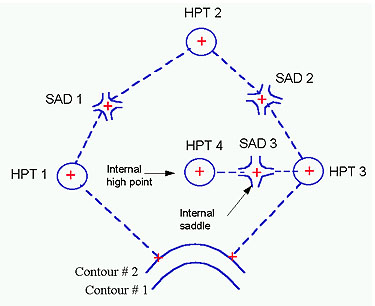
If there are any internal high points and saddles in your catchment, it is necessary to supply extra information to Topog_Element so that an internal watershed may be calculated. This is achieved by building an .iws file. For each internal watershed, the .iws file lists a saddle number, then the number of the two high points forming the ridges to the saddle. The saddle must be an internal saddle and must not have been specified in the .vrt file. The saddle must be listed first, followed by the two peaks in either order. An example of an internal watershed is depicted in the schematic diagram (Figure 3.3) of a catchment shown below.Figure 3.3: Schematic diagram of a catchment depicting an internal watershed.
To represent the internal watershed shown above, the .iws file would contain three lines for each internal watershed. For instance, either:
3 saddle number (internal)
4first-connecting-high point number (internal)
3second-connecting-high point number (boundary) OR
3 saddle number (internal)
3first-connecting-high point number (boundary)
4second-connecting-high point number (internal) The .iws file can be built manually, as above, or automatically using program Topog_Mkbdy. To build one automatically, the steps you need to take are as follows:
- Plot the .tcn file on the screen using Topog_Display.
- Press the Digitise button (see section 6.4.15 for details of how to use this).
- Digitise the start point, high points, saddles and finish point as you would to build the .hpt, .sad and .vrt files as described above in section 3.6. This time, instead of saving the file, press the New Poly button once only and begin by digitising the internal watershed information. Each internal ridge must be added separately to the catchment boundary polygon file. The internal ridges are digitised in sections, each consisting of three points 'High pt-saddle pt-High pt', starting at the high point on the catchment boundary. If there are more than two high points on the internal ridge, then the internal high pts get included in each ridge section as you digitise along the ridge. At the end of each ridge section (3 pts) you press the "New Poly" button once, and do the next one. So for example, if there are 3 high points on the ridge (counting the boundary), then they are digitised :
High pt1-saddle-High pt2 <New Poly>
High pt2-saddle-High pt3 <New Poly>.
When you have digitised all of these, the file can be saved, by
pressing <New Poly/Save> an extra time.Program _mkbdy will detect that internal watersheds exist if more than one line of data is present in the digitised data file.
- Press the New Poly button. After the button title changes to Save, press this; this should result in the writing of a file called basename.dat.a.
3.8 |
Running Topog_Element |
To run Topog_Element, type: $ _elementand supply the basename of your catchment when prompted. Once running, the program automatically seeks out all the mandatory and optional input files associated with the supplied basename as listed below:
Mandatory input files:
basename.sys data bounds file
basename.tcncontours file
basename.hpthigh points file
basename.vrtboundary vertices file
Optional input files :
basename.sad saddles file
basename.iwsinternal watershed file
basename.stlvalley heads file
There are only two further inputs required from the user at the program prompt line, these being the site latitude and the nominal trajectory spacing (nint).
Specify the site latitude in degrees with a + sign for catchments in the northern hemisphere, and a - sign for catchments in the southern hemisphere.
The nint value is the nominal spacing between trajectories. These are calculated along each contour in a sequential manner, starting at the lowest contour, searching upslope at set intervals along this contour, and then moving to the next contour and repeating the process until the uppermost contour is reached. However, the program needs to know how often to create a trajectory, so we instruct it by supplying the nint value. The value you supply will usually be somewhere between 4 and 10; the number relates to the number of points along the contour line (remember that contours are represented simply as long strings of points). For instance, if you supply an nint value of 5, a trajectory will nominally be calculated from every fifth point along the contour.
The true trajectory spacing (in metres on the ground) will vary from catchment to catchment, depending upon the density of points used to represent the contour lines. Thus when you supply the nint value, the program determines the resultant spacing in metres and prompts the user for approval. An excerpt from a typical session is shown below:
The zoom view of the element network (Figure 3.4) shown below illustrates how trajectories converge and diverge according to the shape of the terrain.
Figure 3.4: Zoom view of element network.
Topog_Element displays the catchment boundary, streamlines, ridgelines and trajectories as they are being calculated. If there are any errors, you can usually see where they occur on the screen. Most errors relate to calculation of the boundary and normally result where there is a conflict between a contour height and a high point or saddle elevation. If there is a failure, you may need to return to Topog_Display, display all input files and discern where the error lies.
If everything works, the program will then output a number of files as listed below:
Output files:
basename.sbd catchment boundary
basename.scn catchment contours
basename.stj ends of the trajectories
basename.cct element connections
basename.scct stream element connections (optional)
basename.rdline calculated ridgelines (optional)
basename.stline calculated streamlines (optional)
basename.elm element outlines
basename.atr element attributes
At this stage, it is advisable to backup all of the files you have created. Now that the terrain analysis has been completed, steady state and dynamic water balance analyses can be conducted. Procedures for these are described in Chapter 4 and Chapter 5, respectively.
| Take me out of frames | ..... on to Chapter 4 |