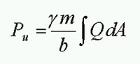
The uniform excess stream power index (P_u) is a parameter used to describe the erosion/energy potential of Hortonian overland flow. It is calculated as the product of overland flow discharge and slope; this is referred to in the literature as mean stream power per unit length of flow (P). In this simulation we assume the whole catchment to be impervious, and we dump a rainfall excess rate (Q) in mm/d over the catchment. The formula used in Topog_Simul to calculate uniform excess stream power is as follows:

4.3

where m is slope (m/m), b is element bottom contour width (m) and g is the specific weight of the fluid and is assumed to be 1. Results are written to a .usp file. The parameter P_u is expressed in units of watts/m².

The variable excess stream power index (P_v) is analogous to the uniform excess stream power index (P_u), except that it is only calculated in areas deemed to be saturated in a previous drainage index simulation. This means that the rainfall excess (Q) is applied only to those elements where the W index is <= 1. However, it is again the mean stream power (P) that is calculated.

The user has the option to run either the normal steady-state drainage index or the radiation-weighted drainage index to set the initial conditions. Go through the steps as outlined in sections 4.2 and 4.3, then specify a rainfall excess as described in section 4.4.

Results are written to a .vsp file. The parameter P_v is expressed in units of watts/m².

The erosion hazard index (H) is based on the variable excess stream power index, but allows you to modulate the calculated energy potential with a variable cover distribution. As with P_u and P_v, H is mapped in units of watts/m², and may be considered as an index of the energy available for the entrainment of sediment.

The erosion hazard index assumes that holding all other factors constant, erosion hazard is related to surface cover in a negative exponential manner. It is based on the findings of Rose (1985) who showed that the efficiency of entrainment of particles by overland flow (h) is primarily a function of surface cover, and may be calculated as:

h = b1 exp [ -b2 (1-Cr)]

4.4

where C_r is the fraction of soil exposed (0-1), and b₁ and b₂ are constants derived empirically from soil loss plot data. Rose (1985) cites a range of b1 values between 0.2 and 0.7 for various cultivated soils in semi-arid Queensland. Values ofC_r, b₁ and b₂ may be distributed as variable quantities across the catchment using Topog_Overlay.

The erosion hazard index H is then calculated as

H = Pu h or H = Pv h

4.5

depending on whether the user chooses to calculate the erosion hazard index using uniform or variable excess stream power (see sections 4.4 and 4.5). Results are written to a .ehi file. More information on the erosion hazard index can be obtained from Vertessy et al. (1990).

Saturation Flow shear stress (t_b) is the boundary shear stress for a given element due to saturation overland flow. It is based on equations developed by Dietrich et al. (1992) and Prosser and Abernethy (1996). The formula used for computing t_b is written as:

tb = ( g2 k r3 8 nc ) 1/3 m2/3 (q a b - Tm )( 2 + c ) / 3

4.6

where g is acceleration due to gravity, r is the density of water (assumed to be 1 gm/cm³), n the viscosity of the fluid (assumed to equal 0.01 cm²s^-1), m = sin(q) where tan(q) is local gradient, q is net lateral drainage flux (see 4.2), a is upslope catchment area and b lower contour width. k and c are defined by empirical relationships between the Darcy-Weisbach friction factor (f) and Reynolds number (Re)

f = k Rec

4.7

where all terms shown are as previously defined. Results are written to a .sss file. The parameter t_b is expressed in units of dynes/cm².

Hortonian shear stress (t_b) is the boundary shear stress for a given element due to Hortonian overland flow: that is, assuming uniform rainfall excess per unit area,

q = R - I

where R is rainfall and I is steady-state infiltration. It is based on the findings of Prosser and Abernathy (1996). The formula used for computing t_b is written as:

tb = ( g2 k r3 8 nc ) 1/3 m2/3 (q a b )( 2 + c ) / 3

4.8

where all terms shown are as previously defined, except that q is now uniform rainfall excess rather than net lateral drainage flux as in 4.6. Results are written to a .hss file. The parameter t_b is expressed in units of dynes/cm².

Landslide hazard index (R_cr) is the minimum steady state rainfall predicted to cause instability (i.e.: the minimum rainfall necessary to cause landslides). It is based on the findings of Montgomery and Dietrich (1994), and is defined as

Rcr = T sin q rs rw [ a b ]-1 [ 1- tan q tan j ]

4.9

where r_s is the bulk density of soil, r_w is the bulk density of water, j the angle of internal friction of soil, and all other terms are as defined previously. Results are written to a .lhi file. The parameter q_cr is expressed in mm/day.