|
|
Chapter 3 |
|
Running the Terrain Analysis System |
|
Sections 3.1 to 3.5 |
3.1 |
Background |
Now that a contour map has been generated which suits your specifications, we can go about segmenting that map and calculating a suite of topographic attributes. This is done with Topog_Element. This program reads in the .tcn file and,
- calculates a catchment boundary from a pair of points on a lower contour
- deletes all parts of contours outside the catchment area
- calculates internal watersheds if they exist
- performs a primary segmentation of the catchment by calculating a network of streamlines and ridgelines, thus partitioning the catchment into a series of hillsides
- performs a secondary segmentation of the catchment by calculating flow trajectories from one contour height to the next upslope, arranged around the previously calculated streamlines and ridgelines
- calculates slope, aspect, and potential solar radiation for various times of the year, for each catchment element, defined by the contour and trajectory network.
Before running Topog_Element, the following parameter files need to be built.
- The high points file (.hpt): specifies the x,y,z coordinates of each discrete high point in the catchment. This file is mandatory.
- The saddles file (.sad): specifies the x,y,z coordinates of each discrete saddle in the catchment. This file is optional.
- The boundary vertices file (.vrt): specifies the start and finish points for the catchment boundary, and the list of high points and saddles the boundary must pass through. This file is mandatory.
- The stream lines file (.stl): lists the co-ordinates of stream heads, used in the primary discretization of the catchment. This file is optional.
- The internal watersheds file (.iws): provides additional boundary information for situations where the catchment has an internal watershed. This file is optional.
Procedures for building the .hpt, .sad, .vrt, .stl and .iws files are described below.
3.2 |
The high points (.hpt) file |
The .hpt file lists the x, y and z coordinates for every high point in the catchment. Each high point is listed on a new line, as shown below.
This file can be built manually, or automatically using program Topog_Mkbdy (see section 3.6 for instructions on how to use this).
To build the file manually, display your .tcn file using Topog_Display. Then use the search button (see section 6.4.11) to establish the x, y coordinates in the centre of all closed contours (make sure you read the absolute coordinate, not the nearest coordinate on a contour). The z value you ascribe to each of these points should be fractionally larger than the contour surrounding it. However, take care to make it less large than the contour interval. For example, if you are putting a high point within a 700 m contour and the contour interval is 2 m, make the z value equal to 701 m.
High points do not have to be listed in any particular order but we recommend that they be listed in sequence, moving anti-clockwise around the catchment boundary. This will make it easier to construct a .vrt file (see section 3.4).
3.3 |
The saddles (.sad) file |
The .sad file lists the x, y and z coordinates for every saddle in the catchment. It has exactly the same structure as the .hpt file, described in section 3.2. A .sad file is only needed if you have more than one high point defined for your catchment.This file can be built manually, or automatically using program Topog_Mkbdy (see section 3.6 for instructions on how to use this).
To build the saddles file manually, follow the same instructions as for the high points file (see section 3.2). However, in the case of saddles, the z value must lie between the elevations of the low and high contours surrounding the saddle. For instance, if the saddle has a low contour value of 800 m and a high contour value of 802 m, then the saddle z value should be defined as 801 m.
As with high points, saddles do not have to be listed in any particular order, but we recommend that they be listed in sequence, moving anti-clockwise around the catchment boundary. This will make it easier to construct a .vrt file (see section 3.4).
3.4 |
The boundary vertices (.vrt) file |
For Topog_Element to calculate a catchment boundary, the user must specify the co-ordinates of boundary start and finish points and a list of high points and saddles for the boundary to pass through. This is done by building a .vrt file.Figure 3.1 shows a schematic representation of a catchment, indicating the components of a .vrt file.
Figure 3.1: Schematic representation of a catchment, indicating the components of a .vrt file. 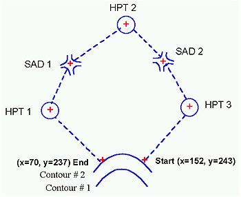
The .vrt file for the catchment shown above would look like this:
2 152. 243.
low-contour-number / x-coord / y-coord (i.e.: boundary start point)
5
total number of high points and saddles to be listed in this file
hpt
flag for a highpoint
3
high point number 3 (i.e.: third point in .hpt file)
sad
flag for a saddle
2
saddle point number 2 (i.e.: second point in .sad file)
hpt
flag for a highpoint
2
high point number 2 (i.e.: second point in .hpt file)
sad
flag for a saddle
1
saddle point number 1 (i.e.: first point in .sad file)
hpt
flag for a high point
1
high point number 1 (i.e.: first point in .hpt file)
2 70. 237.low-contour-number / x-coord / y-coord (i.e.: boundary end point) The low-contour-number is the contour you wish to select as the bottom contour. Let's assume that your .tcn file has contours starting at 100 m with 1 m intervals. Should you wish to start your catchment boundary at 102 m, the starting contour number will be 3. DO NOT use the actual height in metres of the contour. Specify the start and end coordinates so that the boundary is calculated in an anti-clockwise direction. Ensure that these are at least 50 m apart, and that they do not reside on a closed contour (i.e.: a sink at the bottom of the catchment). The start and end points must be on the same contour. The high point and saddle numbers need not be sequential, nor need you include the full list of high points and/or saddles in your .hpt and .sad files. Just make sure that they connect to one another in a logical step-wise manner (e.g.: in the schematic diagram (Figure 3.1) above, high point 3 connects to saddle 2, which connects to high point 2, which connects to saddle 1 .. etc.).
The .vrt file can be built manually, or automatically using program Topog_Mkbdy. Go to section 3.6 for instructions on the automated procedure.
To build a .vrt file manually, first plot the .tcn, .hpt and .sad files on the screen using Topog_Display. Then use the mouse to search for desirable start and end coordinates, and assess which high points and saddles to use (and in which order to list them in your .vrt file). See section 6.4.11 for instructions on how to search for coordinates on the computer screen using Topog_Display. Write all of these values down on a piece of paper, then transcribe them to data files on the computer. This is a messy procedure, but it is safe.
3.5 |
The stream lines (.stl) file |
To perform the primary segmentation of the catchment (i.e.: calculate a series of stream and ridge lines), the user must specify the coordinates of all valley heads within the catchment. While it is not mandatory to perform this primary segmentation, it does significantly improve the way Topog_Element breaks up the terrain.The .stl file can be built manually or automatically, using program Topog_Mkbdy. Go to section 3.6 for instructions on the automated procedure.
To build the .stl file manually, run program Topog_Display and plot the .tcn file. Use the mouse tracking facility in this program, search for the contour coordinates closest to the heads of each valley. See section 6.4.11 for instructions on how to search for coordinates on the computer screen using Topog_Display.
The .stl file is structured in free format. It lists the x,y coordinates and contour number (NOT elevation) that each valley head resides on. An example of an .stl file containing two valley heads is given below.
1306. 1175. 45x co-ord / y co-ord / contour number (i.e. 45th contour from bottom) 1224. 1180. 44x co-ord / y co-ord / contour number (i.e. 44th contour from bottom) Note: The x and y values are real. Contour number is an integer value (ie. no decimal point).
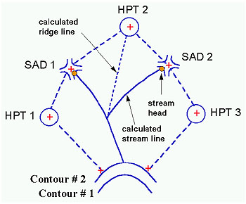
Topog_Element calculates lines downslope from valley heads until the catchment outlet or a stream confluence is reached; these are called calculated streamlines. The program then searches for all confluences and calculates a ridge upslope from these to the nearest high point; these are called calculated ridgelines.
Elements bounding the calculated streamlines are flagged as stream elements. Calculated streamlines are written to an .stline file, while calculated ridgelines are written to an .rdline file. Connections between stream elements are written to a .scct file. A schematic representation (Figure 3.2) of stream head locations and calculated streamlines and bridgelines is shown below.
Figure 3.2: Schematic representation of stream head locations and calculated streamlines and bridgelines.
| Take me out of frames | Chapter 3 continued....... |